
背景
CS231n 看了好几次, 特此整理。大部分参照github仓库 CS231n-2017-Summary
02 Image classification
- Cross-validation 交叉验证, 用来调整超参数
- Split your dataset into
ffolds. - Given predicted hyperparameters:
- Train your algorithm with f-1 folds and test it with the remain flood. and repeat this with every fold.
- Choose the hyperparameters that gives the best training values (Average over all folds)
Linear SVM
- Linear SVM classifier is an option for solving the image classification problem, but the curse of dimensions makes it stop improving at some point.
Logistic regression
- Logistic regression is a also a solution for image classification problem, but image classification problem is non linear!
Logistic Regression 虽然被称为回归,但其实际上是分类模型,并常用于二分类。
“分类”是应用逻辑回归的目的和结果,但中间过程依旧是“回归”。
逻辑回归的损失函数:
\[L=\sum_{i=1}^{n} \log \left(1+\mathrm{e}^{-w^{T} x_{i} y_{i}}\right)\]03 Loss function and optimization
Loss For SVM
L[i] = Sum where all classes except the predicted class (max(0, s[j] - s[y[i]] + 1))
hinge loss 合页损失函数
我们不再把margin的大小作为目标函数,而是考虑分类错误所带来的代价。
对于“+”类()的数据
,我们希望
(同样省略了bias);
对于“-”类(
)的数据
,我们希望
:
总之,我们希望
。
那么,如果实际上
符号为负,或者虽然符号为正但离0不够远,具体来说是
,我们就认为这个分类错误(或“不够正确”)带来了大小为
的损失。
于是目标函数(损失函数)就是
,SVM的训练变成了这个目标函数下的无约束优化问题。
作者:王赟 Maigo链接:https://www.zhihu.com/question/30230784/answer/47837249
-
SVM loss + 正则
Loss = L = 1/N * Sum(Li(f(X[i],W),Y[i])) + lambda * R(W) -
不同的正则化技巧
| Regularizer | Equation | Comments |
|---|---|---|
| L2 | R(W) = Sum(W^2) |
Sum all the W squared |
| L1 | R(W) = Sum(|W|) |
Sum of all Ws with abs |
| Elastic net (L1 + L2) | R(W) = beta * Sum(W^2) + Sum(|W|) |
|
| Dropout | No Equation |
Softmax loss(线性回归做分类,超过两类问题)
softmax function
-
A[L] = e^(score[L]) / sum(e^(score[i]), NoOfClasses)
Softmax loss(真实类别的概率取对数再取负数):
Loss = -logP(Y = y[i]|X = x[i])
Softmax loss is called cross-entropy loss.
\[\frac{\partial C}{\partial z_{i}}=\frac{\partial C}{\partial a_{j}} \frac{\partial a_{j}}{\partial z_{i}}\]Optimization
04. Introduction to Neural network
What is a Computational graphs?
- Used to represent any function. with nodes.
- Using Computational graphs can easy lead us to use a technique that called back-propagation. Even with complex models like CNN and RNN.
Back-propagation simple example:
-
Suppose we have
f(x,y,z) = (x+y)z -
Then graph can be represented this way:
-
X \ (+)--> q ---(*)--> f / / Y / / / Z---------/ -
We made an intermediate variable
qto hold the values ofx+y -
Then we have:
-
q = (x+y)              # dq/dx = 1 , dq/dy = 1
f = qz                 # df/dq = z , df/dz = q
-
-
Then:
-
df/dq = z
df/dz = q
df/dx = df/dq * dq/dx = z * 1 = z       # Chain rule
df/dy = df/dq * dq/dy = z * 1 = z       # Chain rule
-
05. Convolutional neural networks (CNNs)
How Convolutional neural networks works?
-
A fully connected layer is a layer in which all the neurons is connected. Sometimes we call it a dense layer.
- If input shape is
(X, M)the weighs shape for this will be(NoOfHiddenNeurons, X)
- If input shape is
-
Convolution layer is a layer in which we will keep the structure of the input by a filter that goes through all the image.
- We do this with dot product:
W.T*X + b. This equation uses the broadcasting technique. - So we need to get the values of
Wandb - We usually deal with the filter (
W) as a vector not a matrix.
- We do this with dot product:
-
We call output of the convolution activation map. We need to have multiple activation map.
-
Example if we have 6 filters, here are the shapes:
-
Input image
(32,32,3) -
filter size
(5,5,3)- We apply 6 filters. The depth must be three because the input map has depth of three.
-
Output of Conv.
(28,28,6)- if one filter it will be
(28,28,1)
- if one filter it will be
-
After RELU
(28,28,6) -
Another filter
(5,5,6) -
Output of Conv.
(24,24,10)
-
-
-
It turns out that convNets learns in the first layers the low features and then the mid-level features and then the high level features.
-
After the Convnets we can have a linear classifier for a classification task.
-
In Convolutional neural networks usually we have some (Conv ==> Relu)s and then we apply a pool operation to downsample the size of the activation.
-
Number of filters is usually common to be to the power of 2.
# To vectorize well. -
Pooling makes the representation smaller and more manageable.
-
Pooling Operates over each activation map independently.
06. Training neural networks I
Activation functions
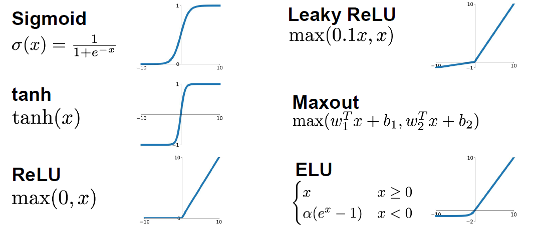
Sigmoid:
- Squashes the numbers between [0,1]
- Used as a firing rate like human brains.
Sigmoid(x) = 1 / (1 + e^-x)- Problems with sigmoid:
- big values neurons kill the gradients.
- Gradients are in most cases near 0 (Big values/small values), that kills the updates if the graph/network are large.
- Not Zero-centered.
- Didn’t produce zero-mean data.
- exp is a bit compute expensive.
- just to mention. We have a more complex operations in deep learning like convolution.
- big values neurons kill the gradients.
Tanh:
- Squashes the numbers between [-1,1]
- Zero centered.
- Still big values neurons “kill” the gradients.
Tanh(x)is the equation.- Proposed by Yann Lecun in 1991.
RELU (Rectified linear unit):
-
RELU(x) = max(0,x) -
Doesn’t kill the gradients.
- Only small values that are killed. Killed the gradient in the half
-
Computationally efficient.
-
Converges much faster than Sigmoid and Tanh
(6x) -
More biologically plausible than sigmoid.
-
Proposed by Alex Krizhevsky in 2012 Toronto university. (AlexNet)
-
Problems:
- Not zero centered.
-
If weights aren’t initialized good, maybe 75% of the neurons will be dead and thats a waste computation. But its still works. This is an active area of research to optimize this.
举例:
假设有一个神经网络的输入W遵循某种分布,对于一组固定的参数(样本),w的分布也就是ReLU的输入的分布。假设ReLU输入是一个低方差中心在+0.1的高斯分布。
在这个场景下:
- 大多数ReLU的输入是正数,因此
- 大多数输入经过ReLU函数能得到一个正值(ReLU is open),因此
- 大多数输入能够反向传播通过ReLU得到一个梯度,因此
- ReLU的输入(w)一般都能得到更新通过随机反向传播(SGD)
现在,假设在随机反向传播的过程中,有一个巨大的梯度经过ReLU,由于ReLU是打开的,将会有一个巨大的梯度传给输入(w)。这会引起输入w巨大的变化,也就是说输入w的分布会发生变化,假设输入w的分布现在变成了一个低方差的,中心在-0.1高斯分布。
在这个场景下:
- 大多数ReLU的输入是负数,因此大多数输入经过ReLU函数能得到一个0(ReLU is close),因此大多数输入不能反向传播通过ReLU得到一个梯度,因此ReLU的输入w一般都得不到更新通过随机反向传播(SGD)
发生了什么?只是ReLU函数的输入的分布函数发生了很小的改变(-0.2的改变),导致了ReLU函数行为质的改变。我们越过了0这个边界,ReLU函数几乎永久的关闭了。更重要的是ReLU函数一旦关闭,参数w就得不到更新,这就是所谓的‘dying ReLU’。
-
To solve the issue mentioned above, people might initialize all the biases by 0.01
Leaky RELU:
leaky_RELU(x) = max(0.01x,x)- Doesn’t kill the gradients from both sides.
- Computationally efficient.
- Converges much faster than Sigmoid and Tanh (6x)
- Will not die.
- PRELU is placing the 0.01 by a variable alpha which is learned as a parameter.
Exponential linear units (ELU):
-
ELU(x) = { x if x > 0 alpah *(exp(x) -1) if x <= 0 # alpah are a learning parameter } -
It has all the benefits of RELU
-
Closer to zero mean outputs and adds some robustness to noise.
-
problems
exp()is a bit compute expensive.
In practice:
- Use RELU. Be careful for your learning rates.
- Try out Leaky RELU/Maxout/ELU
- Try out tanh but don’t expect much.
- Don’t use sigmoid!
Maxout activations:
maxout(x) = max(w1.T*x + b1, w2.T*x + b2)- Generalizes RELU and Leaky RELU
- Doesn’t die!
- Problems:
- oubles the number of parameters per neuron
Data preprocessing
To normalize images:
- Subtract the mean image (E.g. Alexnet)
- Mean image shape is the same as the input images.
- Or Subtract per-channel mean
- Means calculate the mean for each channel of all images. Shape is 3 (3 channels)
Xavier initialization
要求输入的方差等于输出的方差
-
W = np.random.rand(in, out) / np.sqrt(in) -
It works because we want the variance of the input to be as the variance of the output.
- But it has an issue, It breaks when you are using RELU.
He initialization (Solution for the RELU issue):
-
W = np.random.rand(in, out) / np.sqrt(in/2) - Solves the issue with RELU. Its recommended when you are using RELU
Batch normalization:
-
is a technique to provide any layer in a Neural Network with inputs that are zero mean/unit variance.
-
It speeds up the training. You want to do this a lot.
- Made by Sergey Ioffe and Christian Szegedy at 2015.
-
We make a Gaussian activations in each layer. by calculating the mean and the variance.
-
Usually inserted after (fully connected or Convolutional layers) and (before nonlinearity).
-
Steps (For each output of a layer)
-
First we compute the mean and variance^2 of the batch for each feature.
-
We normalize by subtracting the mean and dividing by square root of (variance^2 + epsilon)
- epsilon to not divide by zero
-
Then we make a scale and shift variables:
Result = gamma * normalizedX + beta- gamma and beta are learnable parameters.
- it basically possible to say “Hey!! I don’t want zero mean/unit variance input, give me back the raw input - it’s better for me.”
- Hey shift and scale by what you want not just the mean and variance!
-
-
The algorithm makes each layer flexible (It chooses which distribution it wants)
-
We initialize the BatchNorm Parameters to transform the input to zero mean/unit variance distributions but during training they can learn that any other distribution might be better.
-
During the running of the training we need to calculate the globalMean and globalVariance for each layer by using weighted average.
-
Benefits of Batch Normalization:
- Networks train faster.
- Allows higher learning rates.
- helps reduce the sensitivity to the initial starting weights.
- Makes more activation functions viable.
- Provides some regularization.
- Because we are calculating mean and variance for each batch that gives a slight regularization effect.
-
In conv layers, we will have one variance and one mean per activation map.
-
Batch normalization have worked best for CONV and regular deep NN, But for recurrent NN and reinforcement learning its still an active research area.
-
Its challengey in reinforcement learning because the batch is small.
-
Baby sitting the learning process
- Preprocessing of data.
- Choose the architecture.
- Make a forward pass and check the loss (Disable regularization). Check if the loss is reasonable.
- Add regularization, the loss should go up!
- Disable the regularization again and take a small number of data and try to train the loss and reach zero loss.
- You should overfit perfectly for small datasets.
- Take your full training data, and small regularization then try some value of learning rate.
- If loss is barely changing, then the learning rate is small.
- If you got
NANthen your NN exploded and your learning rate is high. - Get your learning rate range by trying the min value (That can change) and the max value that doesn’t explode the network.
- Do Hyperparameters optimization to get the best hyperparameters values.
Hyperparameter Optimization
- Try Cross validation strategy.
- Run with a few ephocs, and try to optimize the ranges.
- Its best to optimize in log space.
- Adjust your ranges and try again.
- Its better to try random search instead of grid searches (In log space)
07. Training neural networks II
Optimization alogrithms
-
Problems with stochastic gradient descent:
- if loss quickly in one direction and slowly in another (For only two variables), you will get very slow progress along shallow dimension, jitter along steep direction. Our NN will have a lot of parameters then the problem will be more.
- Local minimum or saddle points
- If SGD went into local minimum we will stuck at this point because the gradient is zero.
- Also in saddle points the gradient will be zero so we will stuck.
- Saddle points says that at some point:
- Some gradients will get the loss up.
- Some gradients will get the loss down.
- And that happens more in high dimensional (100 million dimension for example)
- The problem of deep NN is more about saddle points than about local minimum because deep NN has high dimensions (Parameters)
- Mini batches are noisy because the gradient is not taken for the whole batch.
-
SGD + momentum:
-
Build up velocity as a running mean of gradients:
-
# Computing weighted average. rho best is in range [0.9 - 0.99] V[t+1] = rho * v[t] + dx x[t+1] = x[t] - learningRate * V[t+1] -
V[0]is zero. -
Solves the saddle point and local minimum problems.
- It overshoots the problem and returns to it back.
-
-
Nestrov momentum:
-
dx = compute_gradient(x) old_v = v v = rho * v - learning_rate * dx x+= -rho * old_v + (1+rho) * v - Doesn’t overshoot the problem but slower than SGD + momentum
-
-
AdaGrad
-
grad_squared = 0
while(True):
  dx = compute_gradient(x)

  # here is a problem, the grad_squared isn't decayed (gets so large)
  grad_squared += dx * dx

  x -= (learning_rate*dx) / (np.sqrt(grad_squared) + 1e-7)
-
-
RMSProp
-
grad_squared = 0 while(True): dx = compute_gradient(x) #Solved ADAgra grad_squared = decay_rate * grad_squared + (1-grad_squared) * dx * dx x -= (learning_rate*dx) / (np.sqrt(grad_squared) + 1e-7) - People uses this instead of AdaGrad
-
-
Adam
- Calculates the momentum and RMSProp as the gradients.
- It need a Fixing bias to fix starts of gradients.
- Is the best technique so far runs best on a lot of problems.
- With
beta1 = 0.9andbeta2 = 0.999andlearning_rate = 1e-3or5e-4is a great starting point for many models!
first_moment = 0 second_moment = 0 while True: dx = compute_gradient(x) first_moment = beta1 * first_moment + (1 - beta1) * dx second_moment = beta2 * second_moment + (1 - beta2) * dx * dx x -= learning_rate * first_moment / (np.sqrt(second_moment) + 1e-7)) -
Learning decay
- Ex. decay learning rate by half every few epochs.
- To help the learning rate not to bounce out.
- Learning decay is common with SGD+momentum but not common with Adam.
- Dont use learning decay from the start at choosing your hyperparameters. Try first and check if you need decay or not.
-
All the above algorithms we have discussed is a first order optimization.
-
Second order optimization
-
Use gradient and Hessian to from quadratic approximation.
-
Step to the minima of the approximation.
-
What is nice about this update?
- It doesn’t has a learning rate in some of the versions.
-
But its unpractical for deep learning
- Has O(N^2) elements.
- Inverting takes O(N^3).
-
L-BFGS
is a version of second order optimization
- Works with batch optimization but not with mini-batches.
-
-
In practice first use ADAM and if it didn’t work try L-BFGS.
-
Some says all the famous deep architectures uses SGS + Nestrov momentum
Regularization
Model Ensembles:
- Algorithm:
- Train multiple independent models of the same architecture with different initializations.
- At test time average their results.
- It can get you extra 2% performance.
- It reduces the generalization error.
- You can use some snapshots of your NN at the training ensembles them and take the results.
Dropout:
- In each forward pass, randomly set some of the neurons to zero. Probability of dropping is a hyperparameter that are 0.5 for almost cases.
- So you will chooses some activation and makes them zero.
- It works because:
- It forces the network to have redundant representation; prevent co-adaption of features!
- If you think about this, It ensemble some of the models in the same model!
- At test time we might multiply each dropout layer by the probability of the dropout.
- Sometimes at test time we don’t multiply anything and leave it as it is.
- With drop out it takes more time to train.
Dropout 工作流程
假设我们要训练这样一个神经网络,如图2所示。
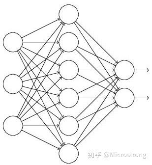 图2:标准的神经网络
输入是x输出是y,正常的流程是:我们首先把x通过网络前向传播,然后把误差反向传播以决定如何更新参数让网络进行学习。使用Dropout之后,过程变成如下:
(1)首先随机(临时)删掉网络中一半的隐藏神经元,输入输出神经元保持不变(图3中虚线为部分临时被删除的神经元)
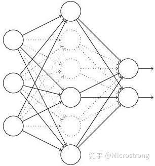 图3:部分临时被删除的神经元
(2) 然后把输入x通过修改后的网络前向传播,然后把得到的损失结果通过修改的网络反向传播。一小批训练样本执行完这个过程后,在没有被删除的神经元上按照随机梯度下降法更新对应的参数(w,b)。
(3)然后继续重复这一过程:
- 恢复被删掉的神经元(此时被删除的神经元保持原样,而没有被删除的神经元已经有所更新)
- 从隐藏层神经元中随机选择一个一半大小的子集临时删除掉(备份被删除神经元的参数)。
- 对一小批训练样本,先前向传播然后反向传播损失并根据随机梯度下降法更新参数(w,b) (没有被删除的那一部分参数得到更新,删除的神经元参数保持被删除前的结果)。
不断重复这一过程。
Data augmentation:
- Another technique that makes Regularization.
- Change the data!
- For example flip the image, or rotate it.
- Example in ResNet:
- Training: Sample random crops and scales:
- Pick random L in range [256,480]
- Resize training image, short side = L
- Sample random 224x244 patch.
- Testing: average a fixed set of crops
- Resize image at 5 scales: {224, 256, 384, 480, 640}
- For each size, use 10 224x224 crops: 4 corners + center + flips
- Apply Color jitter or PCA
- Translation, rotation, stretching.
- Training: Sample random crops and scales:
Drop connect
- Like drop out idea it makes a regularization.
- Instead of dropping the activation, we randomly zeroing the weights.
Transfer learning
Steps of transfer learning
- Train on a big dataset that has common features with your dataset. Called pretraining.
- Freeze the layers except the last layer and feed your small dataset to learn only the last layer.
- Not only the last layer maybe trained again, you can fine tune any number of layers you want based on the number of data you have
| Very Similar dataset | very different dataset | |
|---|---|---|
| very little dataset | Use Linear classifier on top layer | You’re in trouble.. Try linear classifier from different stages |
| quite a lot of data | Finetune a few layers | Finetune a large layers |
08. Deep learning software
Static vs dynamic graphs:
- Optimization:
- With static graphs, framework can optimize the graph for you before it runs.
- Serialization
- Static: Once graph is built, can serialize it and run it without the code that built the graph. Ex use the graph in c++
- Dynamic: Always need to keep the code around.
- Conditional
- Is easier in dynamic graphs. And more complicated in static graphs.
- Loops:
- Is easier in dynamic graphs. And more complicated in static graphs.
09. CNN architectures
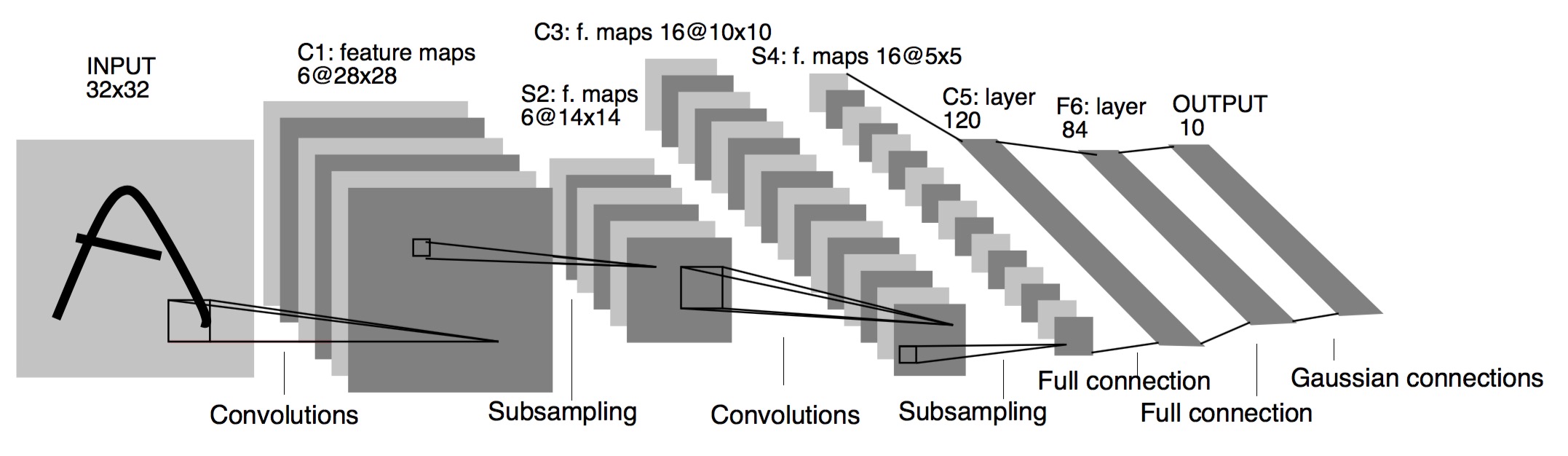
LeNet-5
-
Architecture are:
CONV-POOL-CONV-POOL-FC-FC-FC -
Each conv filters was
5x5applied at stride 1 -
Each pool was
2x2applied at stride2 -
It was useful in Digit recognition.
-
In particular the insight that image features are distributed across the entire image, and convolutions with learnable parameters are an effective way to extract similar features at multiple location with few parameters.
-
It contains exactly 5 layers
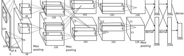
AlexNet
VGGNet
-
The great advantage of VGG was the insight that multiple 3 × 3 convolution in sequence can emulate the effect of larger receptive fields, for examples 5 × 5 and 7 × 7.
-
Used the simple 3 x 3 Conv all through the network.
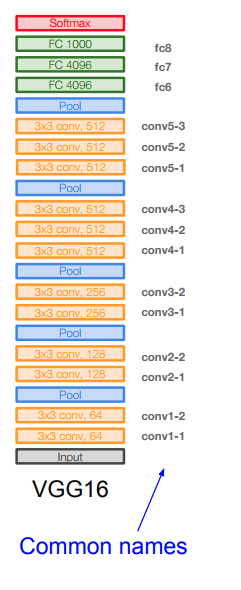
VGG 优点:
在VGG中,使用了3个3x3卷积核来代替7x7卷积核,使用了2个3x3卷积核来代替5*5卷积核,这样做的主要目的是在保证具有相同感知野的条件下,提升了网络的深度,在一定程度上提升了神经网络的效果。
VGG 缺点:
- VGG耗费更多计算资源,并且使用了更多的参数(这里不是3x3卷积的锅),导致更多的内存占用(140M)。其中绝大多数的参数都是来自于第一个全连接层
GoogleNet
TODO
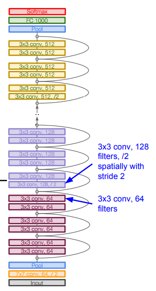
Resnet
如果深层网络后面的层都是是恒等映射,那么模型就可以转化为一个浅层网络。那现在的问题就是如何得到恒等映射了。
152-layer model for ImageNet. Winner by 3.57% which is more than human level error.
This is also the very first time that a network of > hundred, even 1000 layers was trained.
Swept all classification and detection competitions in ILSVRC’15 and COCO’15!
What happens when we continue stacking deeper layers on a “plain” Convolutional neural network?
- The deeper model performs worse, but it’s not caused by overfitting!
- The learning stops performs well somehow because deeper NN are harder to optimize!
The deeper model should be able to perform at least as well as the shallower model.
A solution by construction is copying the learned layers from the shallower model and setting additional layers to identity mapping.
Residual block:
-
Microsoft came with the Residual block which has this architecture:
-
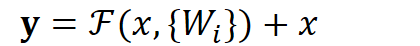
# Instead of us trying To learn a new representation, We learn only Residual
Y = (W2* RELU(W1x+b1) + b2) + X
图中右侧的曲线叫做跳接(shortcut connection),通过跳接在激活函数前,将上一层(或几层)之前的输出与本层计算的输出相加,将求和的结果输入到激活函数中做为本层的输出。
用数学语言描述,假设Residual Block的输入为
,则输出
等于:

其中
是我们学习的目标,即输出输入的残差
。以上图为例,残差部分是中间有一个Relu激活的双层权重,即:

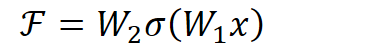
其中
指代Relu,而
指代两层权重。
顺带一提,这里一个Block中必须至少含有两个层,否则就会出现很滑稽的情况:


显然这样加了和没加差不多……
-
Say you have a network till a depth of N layers. You only want to add a new layer if you get something extra out of adding that layer.
-
One way to ensure this new (N+1)th layer learns something new about your network is to also provide the input(x) without any transformation to the output of the (N+1)th layer. This essentially drives the new layer to learn something different from what the input has already encoded.
- The other advantage is such connections help in handling the Vanishing gradient problem in very deep networks.

10. Recurrent Neural networks
So what is a recurrent neural network?
- Recurrent core cell that take an input x and that cell has an internal state that are updated each time it reads an input.
Recurrent NN Computational graph: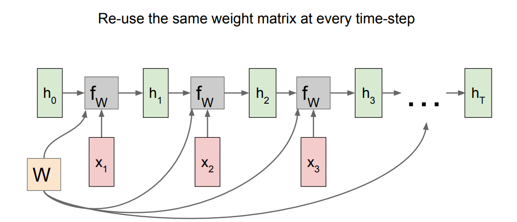
h0are initialized to zero.- Gradient of
Wis the sum of all theWgradients that has been calculated!
LSTM
LSTM stands for Long Short Term Memory. It was designed to help the vanishing gradient problem on RNNs.
- f: Forget gate, Whether to erase cell
- i: Input gate, whether to write to cell
- g: Gate gate (?), How much to write to cell
- o: Output gate, How much to reveal cell
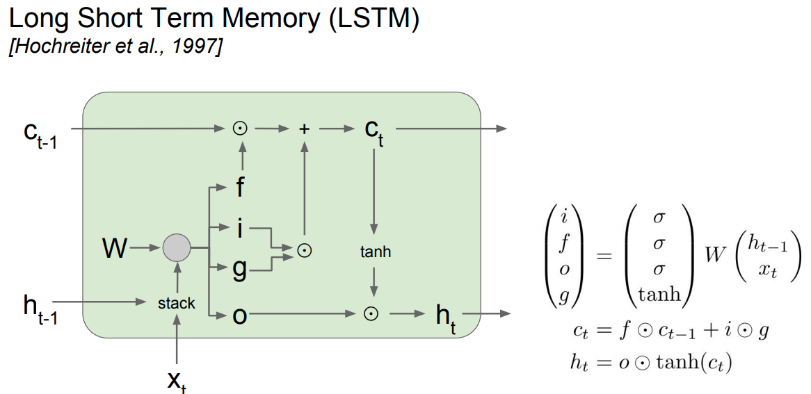

- The LSTM gradients are easily computed like ResNet
- The LSTM is keeping data on the long or short memory as it trains means it can remember not just the things from last layer but layers.
11. Detection and Segmentation
上采样的方法
-
最近邻
Input: 1 2 Output: 1 1 2 2 3 4 1 1 2 2 3 3 4 4 3 3 4 4 -
Bed of Nails 钉床函数:
Input: 1 2 Output: 1 0 2 0 3 4 0 0 0 0 3 0 4 0 0 0 0 0 -
Max unpooling is depending on the earlier steps that was made by max pooling. You fill the pixel where max pooling took place and then fill other pixels by zero.
-
Transpose Conveolution 转置卷积
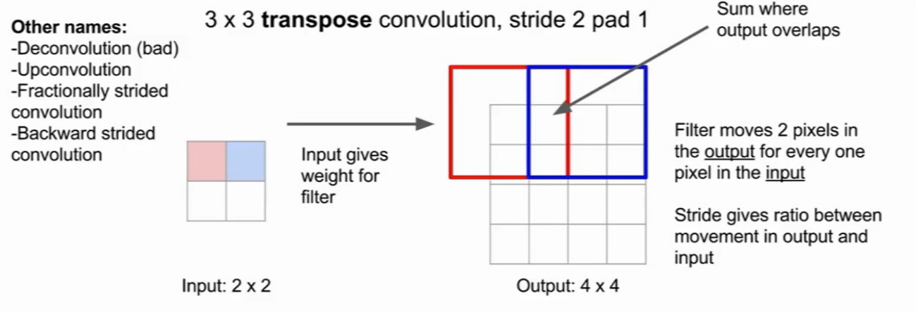
为什么是optput 相加?根据转置卷积的定义: 卷积的转置。
Object Detection
Sliding window
不太现实,因为不知道物体的尺寸与位置
Region Proposals
Selective search. 传统方法,在两秒内提供2000个候选包围框
RCNN
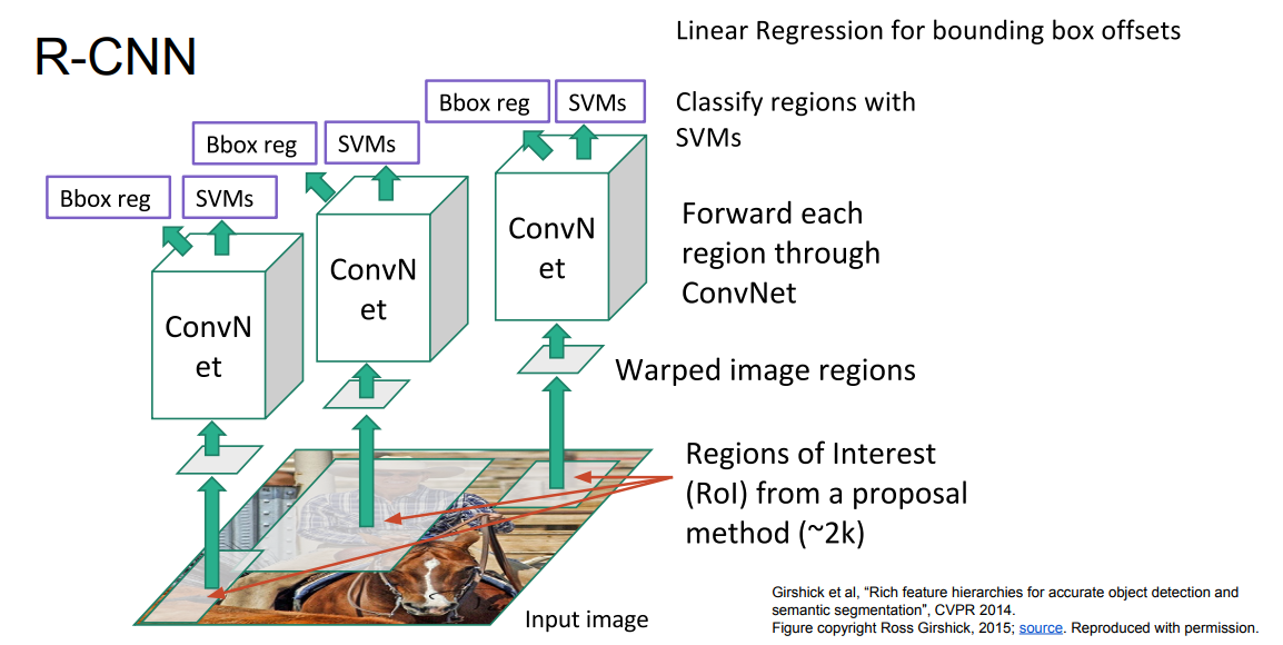
- 用Selective Search 在图像上提取候选框
- 然后对候选框李的图像,先进行卷积,再用SVM做分类得到类别,用回归网络得到当前包围框的修正值
- 训练很慢
- 前向传播也很慢
Fast R-CMM
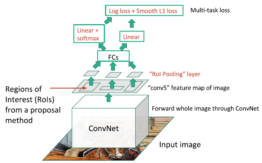
- 对整幅图像进行卷积
- 先获得特征层,随后用类似Selective Search的方法在特征层上提取包围框
- 随后通过全连接层压缩特征,再做分类以及包围框的回归
- 前向推理时,时间主要花在了找候选框上(约2s)。
Faster R-CNN
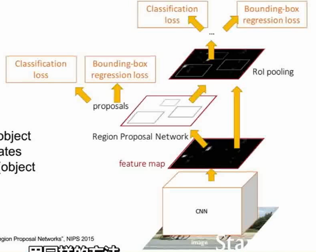
- 用一个 Region Proposal Network 而不是Selective Search来提取包围框。
- 0.2s 一帧
YOLO/SSD
将图像分成7*7的网格。直接一次性回归出包围框的位置与类别,而不是分成两个网络去预测。
Takeaways
- Faster R-CNN is slower but more accurate.
- SSD/YOLO is much faster but not as accurate.
Instance Segmentation 实例分割
Mask R-CNN

12. Visualizing and Understanding
尝试理解卷积网络究竟做了什么事情。
A first approach is to visualize filters of the first layer.
- Maybe the shape of the first layer filter is 5 x 5 x 3, and the number of filters are 16. Then we will have 16 different “colored” filter images.
- It turns out that these filters learns primitive shapes and oriented edges like the human brain does.
- These filters really looks the same on each Conv net you will train, Ex if you tried to get it out of AlexNet, VGG, GoogleNet, or ResNet.
- This will tell you what is the first convolution layer is looking for in the image.
In AlexNet, there was some FC layers in the end. If we took the 4096-dimensional feature vector for an image, and collecting these feature vectors.
- If we made a nearest neighbors between these feature vectors and get the real images of these features we will get something very good compared with running the KNN on the images directly!
- This similarity tells us that these CNNs are really getting the semantic meaning of these images instead of on the pixels level!
- We can make a dimensionality reduction on the 4096 dimensional feature and compress it to 2 dimensions.
- This can be made by PCA, or t-SNE.
- t-SNE are used more with deep learning to visualize the data. Example can be found here.
Visualizing Activations
可以使得中间的特征层被可视化
- For example if CONV5 feature map is 128 x 13 x 13, We can visualize it as 128 13 x 13 gray-scale images.
- One of these features are activated corresponding to the input, so now we know that this particular map are looking for something.
- Its done by Yosinski et. More info are here.
Occlusion Experiments
- We mask part of the image before feeding to CNN, draw heat-map of probability (Output is true) at each mask location
- It will give you the most important parts of the image in which the Conv. Network has learned from.
Saliency Maps
Saliency Maps tells which pixels matter for classification
- Like Occlusion Experiments but with a completely different approach
- We Compute gradient of (unnormalized) class score with respect to image pixels, take absolute value and max over RGB channels. It will get us a gray image that represents the most important areas in the image.
- This can be used for Semantic Segmentation sometimes.
DeepDream: Amplify existing features
- Google released deep dream on their website.
- What its actually doing is the same procedure as fooling the NN that we discussed, but rather than synthesizing an image to maximize a specific neuron, instead try to amplify the neuron activations at some layer in the network.
- Steps:
- Forward: compute activations at chosen layer.
# form an input image (Any image) - Set gradient of chosen layer equal to its activation.
- Equivalent to
I* = arg max[I] sum(f(I)^2)
- Equivalent to
- Backward: Compute gradient on image.
- Update image.
- Forward: compute activations at chosen layer.
- The code of deep dream is online you can download and check it yourself.